I recently built an inference benchmark around a transformer autoencoder, just to teach myself a little about performance engineering fundamentals.
Overview and motivations
During my summer internship, I was training transformer autoencoder models for time-series forecasting and anomaly detection.
There was a pressing need to serve those models at low latencies, so we can make fast decisions based on the results of the models. I was primarily working with time-series data, so a few thousand time windows will come in at the start of every minute and the models would have to score all of them within a couple of seconds— using a 12-hour history of 720 observations and about 32 features per time window.
The model has approximately one million parameters, with about 5 transformer blocks, but the size of the model did not necessarily make the workload cheap, given the latency demands. Here, I discuss some optimisations I tried out to reduce inference latency on both CPUs and GPUs.
CPU Inference
At first, I did not have any GPUs to work with, so I worked on optimising these models for CPU inference. For the most part, these models don't really require GPUs for inference as the model has relatively few parameters and scoring is quite infrequent. On an eight-CPU allocation, the initial FP32 implementation using explicit attention calculations took ~45s to complete a scoring cycle. Using PyTorch's native transformer layers brought that down to ~20s.
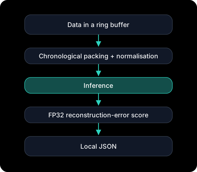
This is what the scoring path looked like:
Making storage updates cheaper
Before optimising model execution, I looked at how the inputs were maintained. Each data source maintains its latest 720 observations. Shifting every data source's history whenever a new observation arrives moves data that has not changed.
A ring buffer avoids this issue. Every minute, the new observation overwrites the oldest slot and the start pointer is advanced to the next oldest entry. Before inference, the buffer is read from that pointer to the end, then from the beginning, producing a chronological sequence in a reusable input buffer.
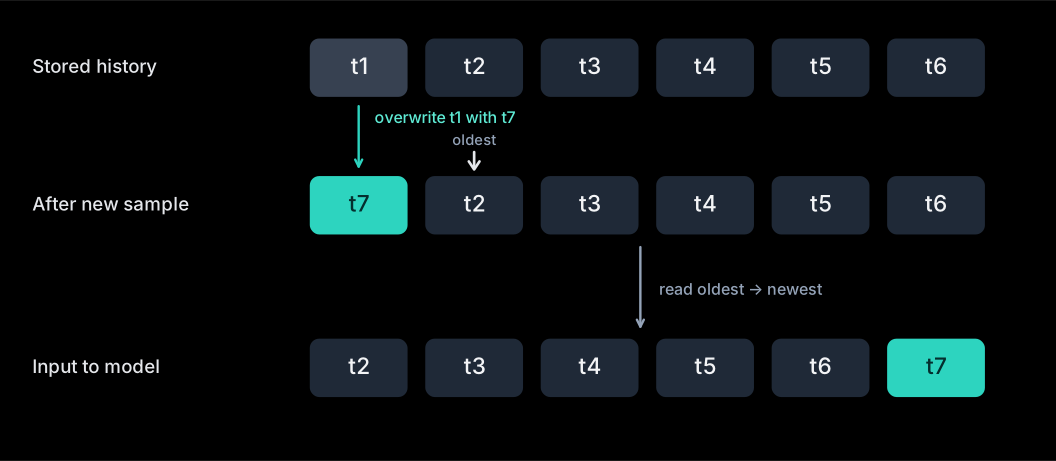
This made history updates much cheaper, from 30.8ms with using an array roll to 0.057ms with circular storage.
CPU performance experiments
For my experiments, I used 8 CPUs and 32GB of RAM. In a matched comparison, native PyTorch transformer layers completed the scoring cycle in 20 seconds, compared with 15 seconds for my tuned scaled-dot product attention (SDPA) path.
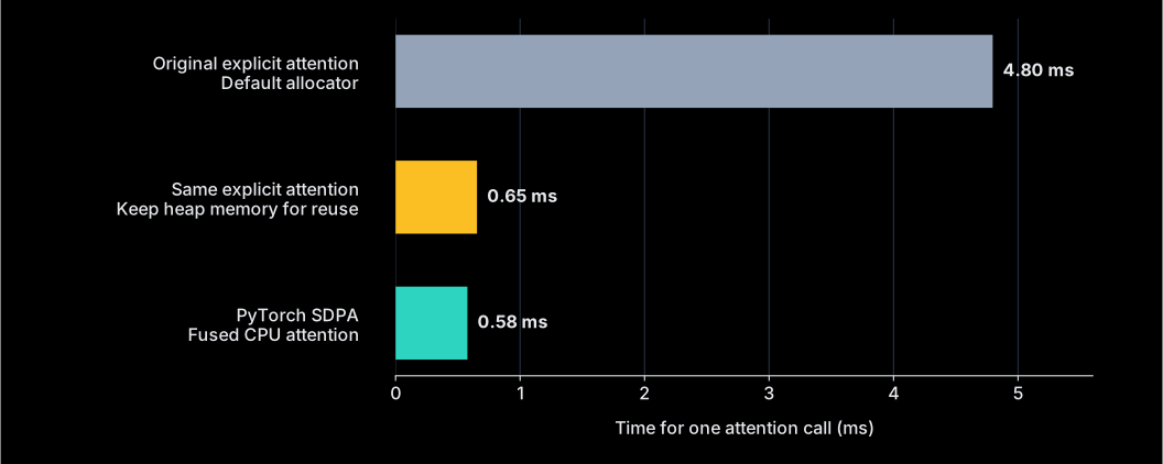
I thought PyTorch’s native transformer layers already use SDPA, so I tried to investigate why this could be the case. Turns out my assumption wasn't always true. In these captures, the native fastpath selected multi-head attention with separate matrix multiplications and softmax. Disabling that fastpath made the same stock layer use fused CPU SDPA, bringing its timing close to my direct-SDPA implementation.
Separately, I investigated why explicit attention was expensive (~45s). It creates large temporary tensors, and releasing their storage can cause the allocator to return memory to the operating system. Subsequent allocations may then incur allocation and page-fault costs. Keeping heap memory available for reuse reduced attention-only latency from 4.80 ms to 0.65 ms, an 86% reduction, without changing the calculation.
I also tested how to distribute windows across the CPU budget. One worker with eight threads lets those threads cooperate on each inference; eight single-thread workers process independent windows concurrently. The latter achieved 171 windows/s, compared with 119 windows/s for the former, approximately 43% more throughput. For this workload, independent inference workers were more effective than additional threads per inference, consistent with coordination costs limiting the benefit of multithreading.
These changes improved CPU execution, but the tested configuration still took approximately 15 seconds to score all 3,000 windows— so I tried some experiments with a GPU to speed things up even further.
GPU performance experiments
Life's good when you get access to a free GPU, you can do some really cool stuff. I used an RTX Pro 4000 Blackwell SFF GPU, with 24GB VRAM. The workload is an innate candidate for parallelism: source windows are independent of one another, many are ready to be inferenced together, and each window contains enough projection and attention work to batch. There is no token-by-token autoregressive generation loop, like LLMs.
Compiled FP32 PyTorch completed the 3,000-window burst in 1.40 seconds. Quantising it to BF16, reduced it even further to 0.32 seconds. Next, I tried tuning batch sizes and transfer strategies.
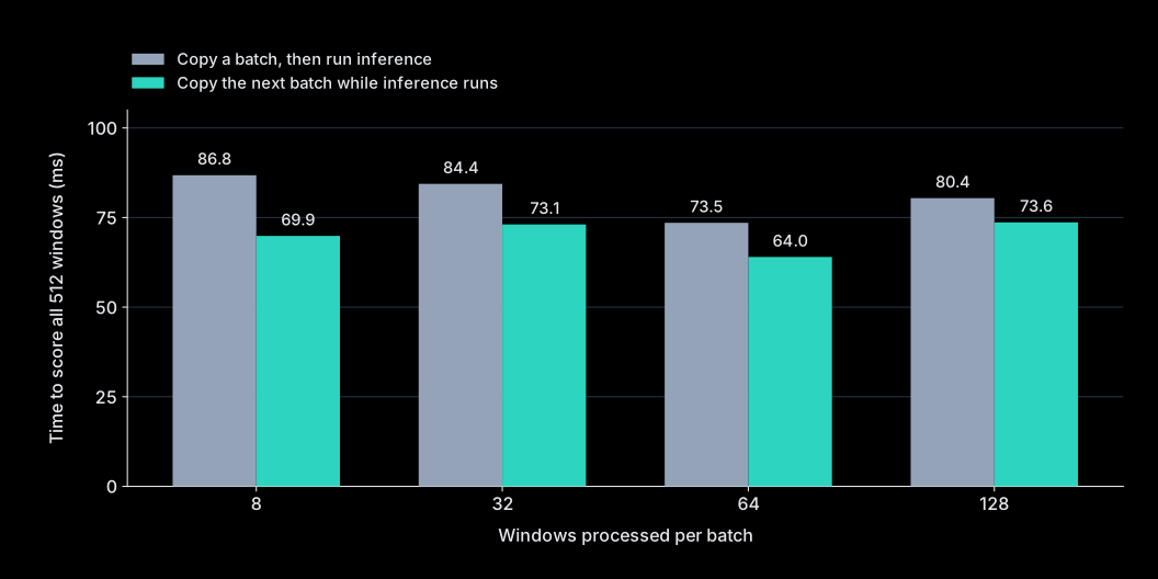
For this comparison, each run scored 512 windows in total. At batch size 64, that meant eight batches of 64 windows each. Reusable pinned buffers and overlapping copies reduced the time to process all 512 windows from 73.5 ms to 64.0 ms, approximately a 13% reduction.
Pinned memory is host memory that the operating system keeps resident in RAM, allowing asynchronous transfers to the GPU. Reusing these buffers also avoids repeatedly allocating and pinning memory for each batch. In the sequential version, each batch was copied to the GPU and then processed before the next copy began. With pipelining, the next batch could be transferred while the GPU was still running inference on the current one, hiding some of the transfer time behind computation.
This requires careful coordination and some strict dependencies. For example, inference had to wait until the copy of its input buffer finished, and buffers could only be overwritten once the operations using them had completed. Without these, a faster pipeline could produce incorrect results by reading incomplete or overwritten inputs.
A batch size of 64 was found to be most optimal. Increasing the batch size to 128 reduced the number of batches to four, but increased total time to 73.6 ms even with overlapping copies. Larger batches can reduce per-batch overhead, but they also change kernel efficiency, memory requirements, and the balance between transfer and compute.
Custom kernels for feed-forward network
After improving compilation and batching, I targeted the feed-forward network (FFN). The formula is as shown:
Executing the 2 projections and GELU operations separately can mean writing full intermediate activation tensors to GPU memory and reading them back for the next operation.
I implemented a fused Triton kernel combining these 3 operations. In this implementation, temporary values can be computed and consumed within the same kernel, avoiding those full intermediate tensors and reducing memory traffic.
I rearranged the weights once into the layout the kernel expects (transposed and contiguous layout), then reused those buffers. Rather than calculate the entire expanded representation at once, the kernel works through it in smaller chunks.
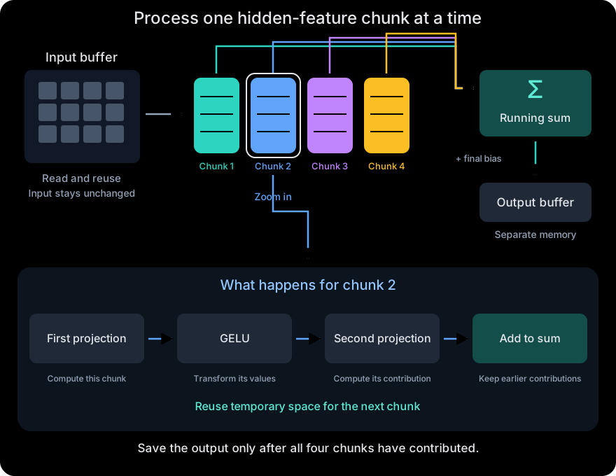
For each chunk, it applies the first projection and GELU, then immediately uses that result in the second projection. Each contribution is added to a running sum. Once every chunk is processed, the kernel saves the final output. Each intermediate value is calculated once and reused within the worker, avoiding full intermediate tensors being saved to GPU memory and read back by another operation.
The tradeoff is how much temporary data to keep close to the computation. Larger chunks allow more reuse but need more of the GPU's limited fast storage, which can leave room for fewer workers to run at once. Smaller chunks need less storage but introduce more separate work. I benchmarked a small set of configurations to choose a balance for this workload.
Fusion also needed to preserve the intended BF16 rounding boundaries. Matrix multiplications can use FP32 accumulators—the running sums of their products—even when the inputs are BF16. The reference can then round that result to BF16 before GELU. I therefore preserved the reference's rounding points inside the kernel, without needing to write the full intermediate tensors to GPU memory.
The complete FFN unit improved from 0.56 ms to 0.29 ms, approximately 1.89× faster.
Results and conclusion
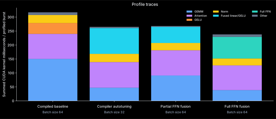
Across randomised rounds with 15 cycles per candidate, the selected custom path averaged 248.46 ms, compared with 323.56 ms for the previous compiled baseline: 23.2% lower latency. I benchmarked against TensorRT as well, which averaged 290ms at a batch size of 32.
The most fun part about this investigation is figuring out how things worked under the hood and figuring out why each change helped reduce the overall latency.
This was a learning project, with room for further optimisation and more work needed before production use. If you have ideas for making it faster, spot something I missed, or want to share feedback, I'd love to hear all about it!
Diagrams generated by Codex.